2013 (Second Generation) Nissan Leaf Drive Unit Teardown

We recently came across a Nissan Leaf drive unit:

Not shown: CHAdeMO charger blob

and of course had to look inside.

First, some outside dimensions for reference:

The drive unit is highly integrated; for example, the motor phase connections are short busbars:

Removing the dozen-odd screws and the three terminal screws allows us to separate the inverter from the motor...

...resulting in a very strange-looking U-shaped motor.

Pulling the next dozen bolts holding the differential and gearbox to the motor separates the gearbox from the motor:

A few more shots of the motor:

The natural next step was to look inside the gearbox...

...which unfortunately meant draining a liter of suspicious red Nissan Leaf fluid out first.

After that, it was simple enough to remove yet another dozen screws and split the gearbox housing:

Nothing much to see here, standard single stage helical gear going into an open differential. More pictures:

Overall reduction is a little over 8:1.

Next we look inside the inverter. First, a quick look at the waterblock channels:

Nothing to see here, standard cast channels.

Cracking the power electronics enclosure open required breaking through a lot of RTV sealant...

...revealing the gorgeous (and never-before-seen!) innards:

The inverter is much less dense than we had anticipated; the IGBT's have their own module (rather than being brazed straight to the waterblock), and there is a lot of empty space over the PM.

Controller is unfortunately based around a datasheet-less Renesas microcontroller, as are all Japanese automotive electronics.

Capacitor is 1088uF, 600V, SH film:

And a lot smaller than the one inside the 2nd-gen Prius.

Few more shots, including gate drive power supplies:

Overall, very well integrated with few surprises. I would not even dream of reprogramming this inverter, as dialing in the motor tuning for something this large would be very involved. My one comment is that this motor is probably good for much more than 80KW peak - judging by its size I would venture to say it is a 200KW-class motor.

Field Weakening, Part 1

Previously on Motor Diddlers, we learned how to optimize the torque produced by an IPM operating in the current-limited regime. We can't stay in this regime forever; at higher RPM's, all motors enter a voltage-limited operating regime.

What's surprising is how quickly IPM's become voltage-limited. Using the data from the last post, we can plot the maximum achievable current versus speed:

The "base speed" of the motor is very low, about 800 rad/s (2500 RPM). Furthermore, we quickly run out of volts past base speed; the motor cannot turn much faster than 1500 rad/s (5000 RPM) if we constrain ourselves to the MTPA trajectory. This is a result of the much higher inductance of an IPM; at high electrical frequencies this inductive impedance limits how much current we can put into the stator.

Fortunately, we can use this higher inductance to our advantage. Recall that \(V_q=R_s I_q+\omega L_d I_d+\omega\lambda\); this means that if \(I_d\) is negative, we can cancel out the \(\omega\lambda\) term (what would conventionally be called "back EMF" in a surface PM machine) in the expression for \(V_q\). On a surface PM machine, this current would be wasted; however, if \(L_d < L_q\), the \((L_d-L_q)I_d I_q\) term in the torque equation will generated positive torque! Furthermore, the \(L_d/\lambda\) ratio is often an order of magnitude higher for IPM's, which greatly reduces the amount of d-axis current required to cancel out the flux linkage. This is, in a nutshell, why IPM's field weaken much better than their surface PM counterparts.

It is fairly straightforward to compute the optimal field-weakening trajectory:

Starting from the motor equations $$
\begin{array}{lcl}
\tau=\frac{3}{2}n_p(\lambda I_q+(L_d-L_q)I_d I_q)\\
V_d=R_s I_d-\omega L_q I_q\\
V_q=R_s I_q+\omega L_d I_d+\omega\lambda\\
V_s=\sqrt{V_d^2+V_q^2}\\
I_s=\sqrt{I_d^2+I_q^2}
\end{array}
$$ we note that in the voltage limited operating regime, maximum torque must be achieved when the voltage vector is on the boundary of the allowable area, in which case the optimization problem becomes an equality: $$
\begin{cases}
\frac{3}{2}n_p(\lambda I_q+(L_d-L_q)I_d I_q) = \tau_0\\
(R_s I_d-\omega L_q I_q)^2 + (R_s I_q+\omega L_d I_d+\omega\lambda)^2 = V_0^2
\end{cases}
$$ If we ignore saturation, this system is the intersection of a constant-torque hyperbola (which is independent of speed) and a series of shrinking ellipses.

This system is polynomial (and in fact only a quartic) and can be solved in many ways. For example, one element of the reduced Groebner basis of the ideal generated by the two equations is the very long $$
(L_d-L_q)^2(R_s^2+L_q^2w^2)I_q^4 +
(L_q^2\lambda^2\omega^2+R_s^2\lambda^2+(L_d-L_q)^2(2R_s\tau_0\omega-V_0^2))I_q^2-
2\lambda\tau_0(R_s^2+L_d L_q\omega^2)+
R_s^2\tau_0^2+L_d^2\tau_0^2\omega^2
$$ where we have included the factor of \(3/2n_p\) in \(\tau_0\) for brevity's sake. The roots of this polynomial are easily found with a variety of numeric or analytic methods; in the case of multiple real solutions the correct one is the \((I_d,I_q)\) vector with the shortest length.
Unfortunately, the system is no longer polynomial if the motor saturates (that is, \(L_d\) and \(L_q\) are functions \(l_d(I_d,I_q)\), \(l_q(I_d,I_q)\) of the axis currents). In order to solve the system in this case, we will have to turn to more complicated (and less reliable) numeric methods, the nature of which will be the subject of the next post in this series.

Focusing on the Ground

Suppose we have a view camera and we wish to focus on a horizontal plane. More precisely, let the center of the lens \(O\) be \(a\) above the ground, and suppose the rear standard makes an angle \(\theta\) with respect to the horizontal. We wish to find the angle \(\alpha\) that the front standard must be tilted at to focus on the ground.

By the Scheimpflug rule. the rear standard, front standard, and horizontal intersect at a point \(S\). By the hinge rule, the front focal plane, the horizontal, and the plane through \(O\) parallel to the rear standard are concurrent; this is true if and only if the intersection point \(H\) of the horizontal and the plane parallel to the rear standard lies at a distance \(f\) from the front standard, where \(f\) is the focal length of the lens.

We have:
\begin{array}{lcl}
O'S = a / \tan{\alpha}\\
O'H = a / \tan{\theta}\\
SH = O'S - O'H = a(1/\tan{\alpha} - 1/\tan{\theta}) = a \left( \frac{\cos{\alpha}}{\sin{\alpha}} - \frac{\cos{\theta}}{\sin{\theta}} \right)
\end{array}
This means:
\begin{array}{lcl}
f = SH\sin{\alpha} = a\sin{\alpha} \left( \frac{\cos{\alpha}}{\sin{\alpha}} - \frac{\cos{\theta}}{\sin{\theta}} \right)\\
\frac{f}{a} = \cos{\alpha}-\frac{\cos{\theta}}{\sin{\theta}}\sin{\alpha}\\
\frac{f}{a}\sin{\theta} = \cos{\alpha}\sin{\theta} - \sin{\alpha}\cos{\theta} = \sin{(\theta-\alpha)}\\
\theta-\alpha = \arcsin{(\frac{f}{a}\sin{\theta})}\\
\alpha = \theta-\arcsin{(\frac{f}{a}\sin{\theta})}
\end{array}
In other words, the angle between the front and rear standards is \(\arcsin{(\frac{f}{a}\sin{\theta})}\). This is pretty neat; in particular, for small magifications we can say the ratio of  of the sines of the angles is approximately equal to the magnification of the camera.

Obligatory 2017 Eclipse GIF

Somehow this endeavor went better than planned, I was able to not only get to the site successfully and make it through traffic, but also get the tracking mount to track.

There was an "urp" moment when I fumbled and disconnected my A7II from the remote shutter app during totality, and another "urp" moment when I panicked and complete forgot about proper exposure times and such, but 1/80 turned out OK and the raw files have enough exposure latitude to do a bit of HDR if need be...

A7II and Celestron C5 w/0.63x focal reducer (~750mm f/6.3), Spectrum glass filter, 1/80s ISO 100

Super Plumbing

The cadet racing kart chassis we were working with had no front brakes. This was a problem, because our stopping power was already traction-limited at the rear wheels, and more time spent stopping meant less time accelerating.

Front brake conversion kits exist, but are rather expensive. Undaunted, we bought some generic moped calipers, proclaiming that "we'll figure out a way to mount them".

Ben came up with a pretty good way to mount them:

The stock direct spindle mount front wheels were replaced with a set of hub-mount rear wheels, and new hubs with 17mm bearings were made to mount them to the spindles. The arm that holds the caliper is centered using the precision-machined spindle shaft (which is the only precision surface in the kingpin assembly). Finally, a cross-piece is made which bolts to the arm and prevents it from rotating around the spindle.

Everything was made on the MITERS CNC (a mid-90's Dyna-Myte converted to LinuxCNC), and the mounts worked great.

The next step was to fill the brakes. Initial attempts were made to drive the two front calipers and the rear caliper (which had two pistons) using a single master cylinder:

Nope

This proved to be exceedingly unsuccessful; not only did the master cylinder have borderline displacement to drive four pistons, getting the air out of the loop and matching the piston travels proved to be nearly impossible. A day and a half into the ordeal, standards were lowered, and we decided to run the front and rear brakes off separate master cylinders actuated by a single pedal.

A word on the hoses: moped calipers take banjo bolts (hollow bolts sealed with crush washers). We used Earl's Performance braided lines to turn these into -3AN flares:

 These connect to a 1/8" NPT tee:

The third arm of the tee is fitted with an NPT-to-compression adapter, which then goes to the master cylinder. A very unconventional setup, as compression fittings are not typically rated to brake line pressures. Go-karts get away with it with a combination of low pressures (hundreds, instead of thousands, of PSI) and short maintenance cycles (typically a couple dozen hours of runtime per season).

IPM Low-Speed Optimization

I had mentioned in a previous post that IPM's require both d and q-axis currents for optimal performance. Thanks to the motor equations, it is easy to quantify this split.

Recall that a sinusoidally-varying motor is modeled by:$$
\begin{array}{lcl}
\tau=\frac{3}{2}n_p(\lambda I_q+(L_d-L_q)I_d I_q)\\
V_d=R_s I_d-\omega L_q I_q\\
V_q=R_s I_q+\omega L_d I_d+\omega\lambda\\
V_s=\sqrt{V_d^2+V_q^2}\\
I_s=\sqrt{I_d^2+I_q^2}
\end{array}
$$ Suppose we have unlimited back EMF, and we wish to optimize torque per amp. There are two ways to look at this. Firstly, we could $$
\mbox{minimize }
\begin{cases}
I_d^2+I_q^2\mbox{ subject to}\\
\lambda I_q+(L_d-L_q)I_d I_q=\tau_0
\end{cases}
$$ Or, we could $$
\mbox{maximize }
\begin{cases}
\lambda I_q+(L_d-L_q)I_d I_q\mbox{ subject to}\\
I_d^2+I_q^2=I_0^2
\end{cases}
$$ As it turns out, the second current-first approach results in much easier math (we only need to solve a quadratic, not a quartic) at the expense of being somewhat less intuitive (it is unclear what current corresponds to what torque).

There are several ways to solve the second problem; we use Lagrange multipliers here. The Lagrangian is $$L(I_d,I_q,u)=\lambda I_q+(L_d-L_q)I_d I_q-u(I_d^2+I_q^2-I_0^2)$$ where \(u\), not \(\lambda\), is the multiplier.
The system of partial derivatives is $$
\begin{cases}
\frac{\partial L}{\partial I_d}=(L_d-L_q)I_q-2I_d u=0\\
\frac{\partial L}{\partial I_q}=(L_d-L_q)I_d-2I_q u+\lambda=0\\
\frac{\partial L}{\partial u}=I_0^2-I_d^2-I_q^2=0
\end{cases}
$$ This system is easily solved by a computer algebra system or by multiplying the first equation by \(I_q\) and the second by \(I_d\), giving $$
\begin{array}{lcl}
I_d=\frac{-\lambda+\sqrt{\lambda^2+8(L_d-L_q)^2I_0^2}}{4(L_d-L_q)}\\
I_q=\sqrt{I_0^2-I_d^2}
\end{array}
$$ where we have picked the signs knowing that \(I_d\) is negative and \(I_q\) is positive.

Armed with this information we can make some plots. Plugging in the HSG data \(L_d=0.0006\), \(L_q=0.0015\). and \(\lambda=0.053\) (units: Henries, Volt-seconds), we have the following plot:

As expected, \(I_d\) is about the same magnitude as \(I_q\) at high currents.

Plumbing Electrons

"Wiring is like plumbing, but for electrons"

                                                                                                                                    -me, 2017

One of the things I've come to dread in any project is wiring. This particular wiring job is by no means stellar, but works well enough to be worth writing about.

Starting at the front:

The steering wheel controls consist of an e-stop and a key switch. The e-stop is wired in series with the +12V line going to the logic and by extension, the 12V supply for the internal gate drives on the power module. Hitting the e-stop shuts down the microcontroller and gate drive, which safely floats the inverter phases.

The key is wired in series with the 12V going to the contactor control line - contactor power does not go through the e-stop. As interrupting high DC link currents damages the contactor, this switch is intended to act as a last line of defense in case the inverter has failed short or otherwise stopped responding to gate drive. In normal fault situations (throttle failure, firmware error) the e-stop suffices.

From the steering wheel, two runs of McMaster 8082K37 shielded cable connect the switches to a power distribution board...

...which I swear is the only reason the go-kart thinks about working at all. The sketchy CNC'ed board replaces what would be an even sketchier mass of wire junctions.

The HV contactor is a Kilovac Csonka EV200:

The datasheet claims it is rated for dozens of interruptions at 500+A but I don't believe it. The precharge resistor is bolted directly across the contactor, which has the benefit of precharging the DC link capacitor whenever the HV connector is plugged in, and the downside of slowly draining the traction pack should the HV connector be left unplugged.

The motors are wired to the inverter via 10AWG silicone wire stuffed inside a copper braid finger-trap shield:

I am not convinced the shield is doing much (it isn't terminated on either end, and terminating it didn't seem to affect noise), but keeping the phase leads in as small of a bundle as possible is important for reducing radiated noise.The shield is sealed to the wire bundle with 3M EPS-300 adhesive backed heatshrink, which upon heating forms a tough, watertight seal glued to the shield and wires.

Moving back to the inverter:

The phase lead bundles are attached to the bus capacitor tabs by zip-ties. As much of the exposed bus bar as possible is covered in liquid electrical tape to reduce the chance of inverter-induced incidents.

The capacitor itself is mounted via standoffs and slotted tabs to the inverter block:

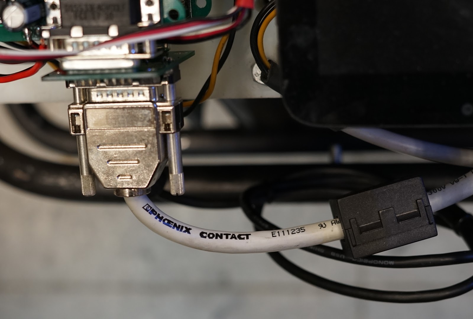
The image above also shows the power module control cable, which is cut short and terminated in a DB-15 connector, then run through a 20" commercial shielded DB-15 cable to the logic board:

The Phoenix Contact cable was irritatingly expensive (~$50 on eBay), but it was rather difficult to find good shielded 15-wire cable.

Finally, the throttle is actuated through a bowden cable attached to the original go-kart throttle pedal (which operated a mechanical throttle on a carbureted engine). The throttle sensor is a GM brake position sensor:

The bowden cable is crimped to a standard copper ring terminal; please don't do this for an actual brake! It is only acceptable here because a cable failure causes the throttle to return to an off-position.